Osciladores LC

Un oscilador muy sencillo se puede construir con una etapa amplificadora y un red inductiva-capacitiva (LC) que proporcione un desplazamiento de -180°.

La frecuencia de oscilación puede ser fácilmente ajustada, o sintonizada (tuned), sobre un rango de frecuencias que varían desde unos 100kHz hasta cientos de MHz cambiando únicamente el valor de la C o L.

Estos osciladores LC sintonizados son usados en gran variedad de aplicaciones incluyendo radiotransmisores, receptores de AM y FM y generadores de onda sinusoidal.

Los osciladores LC más conocidos son: a) oscilador de Colpitts y b) oscilador de Hartley. Su diferencia se encuentra en la red de realimentación: el oscilador de Colpitts utiliza un divisor capacitivo en paralelo con una autoinducción y el oscilador de Hartley utiliza un divisor inductivo en paralelo con una capacidad, es decir, ambos son duales.

En la figura 10.7 se indican tres posibles configuraciones de un oscilador Colpitts basado en transistores FET y BJT, y en un OA aunque no suelen ser utilizado por su limitación en frecuencia; la autoinducción RFC sirve para aislar la línea de alimentación del oscilador, es decir, su valor es suficientemente alto para impedir que la señal sinusoidal se transmita a la alimentación.

Si la frecuencia de oscilación (ƒ_o) es suficientemente baja para considerar despreciable los efectos capacitivos internos de los transistores y el OA, y si la autoinducción L tiene una resistencia interna despreciable, entonces la frecuencia de oscilación será determinada por la red LC (también conocida en muchos casos con el nombre de circuito tanque o tank porque se comporta como una depósito de energía de almacenamiento). Para el oscilador Colpitts, esta frecuencia es

Esta relación debe ser combinada con la ganancia de l a etapa amplificadora para asegurar las condiciones de oscilación.

De la misma manera, la frecuencia de oscilación de los osciladores Hartley mostrados en la figura 10.8 viene dada por

---

Transmisor de CW

La forma más simple de transmisor es el oscilador que muestra la figura 10-1. El oscilador genera una señal portadora
con la frecuencia deseada. La frecuencia aquí está determinada por un cristal. La información que se transmite se expresaen una forma especial de código que utiliza puntos y rayas para representar las letras del alfabeto y los números.
La información transmitida de esta manera se conoce como transmisión de onda continua (CW, continuous wave). En
el emisor se utiliza una llave conveniente, que es un interruptor operado en forma manual para encender y apagar el
oscilador a fin de producir los puntos y rayas. El oscilador produce un breve pulso de energía de RF para un punto y un
pulso de RF más prolongado para una raya. Aun cuando un transmisor tan simple como éste puede tener una potencia
de 1 W o menos, a la frecuencia correcta y con una buena antena es capaz de enviar señales a la mitad del alance mundial (en HF).

El transmisor de CW básico ya descrito puede mejorar en forma considerable agregando un amplificador de potencia.
El resultado se muestra en la figura 10-2. El oscilador se controla con la llave para producir puntos y rayas, pero el amplificador incrementa el nivel de potencia de la señal. El resultado es una señal más intensa que tendrá un alcance mayor y producirá comunicaciones más confiables.

La combinación básica oscilador-amplificador que ilustra la figura 10-2 es la base de casi todos los transmisores de
radio. Según el tipo de modulación que se use, el nivel de potencia y otras consideraciones se agregan muchos otros
circuitos. Los siguientes son algunos de los transmisores que emplean varios tipos de modulación.
Figura 10-2 Transmisor de CW con mayor potencia.

Transmisor de AM
un transmisor de AM, en el que un oscilador genera la frecuencia de la portadora final. En la
mayoría de las aplicaciones se trata de un oscilador a cristal. En general, los transmisores operan con frecuencias o
canales asignados y los cristales proporcionan la mejor forma de obtener la frecuencia deseada con buena estabilidad.
Por lo común, los osciladores LC no tienen la estabilidad de frecuencia requerida para mantenerse en frecuencia. Las
variaciones de temperatura y otras condiciones hacen que la frecuencia salga de los límites que impone la CNC.
La señal de la portadora se envía a un amplificador de aislamiento (buffer) cuya finalidad principal es aislar el oscilador
de las demás etapas de amplificación de potencia. Dicho amplificador de aislamiento por lo general opera en clase
A y proporciona un incremento modesto en la potencia de salida. El propósito principal de ese amplificador es impedir
que los cambios en la carga ocasionen variaciones de frecuencia en el oscilador.
La señal del amplificador de aislamiento (buffer) se aplica al amplificador de excitación. Éste es un amplificador clase
C diseñado para proporcionar un nivel intermedio de amplificación de potencia. La finalidad de este circuito es generar
suficiente potencia de salida para alimentar la etapa de amplificación de potencia final.
El amplificador de potencia final, que se conoce simplemente como el final, también opera en clase C con potencia
muy alta. La cantidad de potencia real depende de la aplicación; por ejemplo, en un transmisor de CB, la potencia de
entrada es de sólo 5 W Sin embargo, las radiodifusoras de AM operan con potencias mucho más altas, de 250, 500,
1000, 5 000 o 50 000 W.
Todos los circuitos de RF del transmisor por lo común son de estado sólido; es decir, se implementan con transistores
bipolares o de efecto de campo. Aun cuando los transistores bipolares son con mucho los más comunes, los MOSFET
se usan más ya que ahora tienen capacidad para manejar alta potencia.

Los transistores a menudo también se emplean en el amplificador final, siempre que el nivel de potencia no exceda de
varios cientos de watts. Los transistores de potencia de RF individuales pueden manejar hasta 300 W. Estos transisto
res se pueden conectar en paralelo o en configuraciones en contrafase (push-pull) para incrementar aún más la capacidad de manejo de potencia. Sin embargo, en los amplificadores finales rara vez se usan transistores, si la salida de potencia excede los 5 000 W. Para niveles de potencia más altos todavía se usan tubos al vacío.
Consideremos que la figura 10-3 es un transmisor de voz. La entrada del micrófono se conecta a un amplificador de
audio clase A de bajo nivel, el cual refuerza la señal pequeña del micrófono a un nivel de voltaje más alto; se pueden
usar una o más etapas de amplificación.
La señal de voz se envía a alguna forma de circuito de procesamiento de voz. "Procesamiento de voz" se refiere al filtrado y control de amplitud. El filtrado asegura que las frecuencias de voz sólo se dejan pasar en determinado intervalo, lo que permite minimizar el ancho de banda que ocupa la señal. La mayoría de los transmisores de comunicaciones limitan la frecuencia de voz al intervalo de 300 Hz a 3 000 Hz, que es el adecuado para comunicaciones inteligibles.
Sin embargo, las radiodifusoras de AM ofrecen una fidelidad más alta y permiten frecuencias hasta de 5 kHz. El procesador de voz también consta de alguna clase de circuito para mantener la amplitud en un nivel particular. Las
señales de amplitud de alto nivel se comprimen y a las señales de nivel más bajo suele dárseles más amplificación; el
resultado es que se impide la sobremodulación. Así se reduce la posibilidad de distorsión de la señal y las armónicas
que producen bandas laterales más anchas que pueden causar interferencia al canal adyacente. (Compandores)
Después del procesador de voz se usa un amplificador de excitación. Este elemento incrementa el nivel de potencia de
la señal para que tenga la capacidad de alimentar el amplificador de modulación de alta potencia. En el transmisor de
AM de la figura 10-3 se usa modulación de alto nivel o de colector. Como ya se mencionó, la potencia de salida del
amplificador de modulación debe ser la mitad de la potencia de entrada del amplificador de RF. El amplificador de
modulación de alta potencia en general opera en clase AB o en clase B en push-pull para alcanzar estos niveles de potencia.

Ricardo A. Monroy B.   C.I. 17646658
EES

---

Darlington transistor

In electronics, the Darlington transistor (often called a Darlington pair) is a compound structure consisting of two bipolar transistors (either integrated or separated devices) connected in such a way that the current amplified by the first transistor is amplified further by the second one.^[1] This configuration gives a much higher current gain (written β, h_fe, or h_FE) than each transistor taken separately and, in the case of integrated devices, can take less space than two individual transistors because they can use a shared collector. Integrated Darlington pairs come packaged in transistor-like packages. The Darlington configuration was invented by Bell Laboratories engineer Sidney Darlington in 1953. He patented the idea of having two or three transistors on a single chip, sharing a collector.^[2]
A similar configuration but with transistors of opposite type (NPN and PNP) is the Sziklai pair, sometimes called the "complementary Darlington."

Circuit diagram of a Darlington pair using NPN transistors

     A Darlington pair behaves like a single transistor with a high current gain approximately the product of the gains of the two transistors). In fact, integrated devices have three leads (B, C and E), broadly equivalent to those of a standard transistor.

A general relation between the compound current gain and the individual gains is given by:

If β₁ and β₂ are high enough (hundreds), this relation can be approximated with:

A typical modern device has a current gain of 1000 or more, so that only a small base current is needed to make the pair switch on. However, this high current gain comes with several drawbacks.

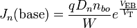
One drawback is an approximate doubling of base-emitter voltage. Since there are two junctions between the base and emitter of the Darlington transistor, the equivalent base emitter voltage is the sum of both base-emitter voltages:

For silicon-based technology, where each V_BEi is about 0.65 V when the device is operating in the active or saturated region, the necessary base-emitter voltage of the pair is 1.3 V.

Another drawback of the Darlington pair is its increased saturation voltage. The output transistor is not allowed to saturate (i.e. its base-collector junction must remain reverse-biased) because its collector-emitter voltage is now equal to the sum of its own base-emitter voltage and the collector-emitter voltage of the first transistor, both positive quantities in normal operation. (In symbols, V_CE2 = V_BE2 + V_CE1, so V_C2 > V_B2 always.) Thus the saturation voltage of a Darlington transistor is one V_BE (about 0.65 V in silicon) higher than a single transistor saturation voltage, which is typically 0.1 - 0.2 V in silicon. For equal collector currents, this drawback translates to an increase in the dissipated power for the Darlington transistor over a single transistor.

Another problem is a reduction in switching speed, because the first transistor cannot actively inhibit the base current of the second one, making the device slow to switch off. To alleviate this, the second transistor often has a resistor of a few hundred ohms connected between its base and emitter terminals.^[1] This resistor provides a low impedance discharge path for the charge accumulated on the base-emitter junction, allowing a faster transistor turn-off.

The Darlington pair has more phase shift at high frequencies than a single transistor and hence can more easily become unstable with negative feedback (i.e., systems that use this configuration can have poor phase margin due to the extra transistor delay).

Darlington pairs are available as integrated packages or can be made from two discrete transistors; Q₁ (the left-hand transistor in the diagram) can be a low power type, but normally Q₂ (on the right) will need to be high power. The maximum collector current I_C(max) of the pair is that of Q₂. A typical integrated power device is the 2N6282, which includes a switch-off resistor and has a current gain of 2400 at I_C=10A.

A Darlington pair can be sensitive enough to respond to the current passed by skin contact even at safe voltages. Thus it can form the input stage of a touch-sensitive switch.

Ricardo A. Monroy B.   C.I. 17646658
EES

---

differential amplifier

Algunas Configuraciones

Three lesser known BJT configurations are the differential amplifier, current mirror and the darlington amplifier. These circuits all require two transistors, which should be the same type and have closely matched parameters for best performance,. For clarity, all circuits are drawn without bias circuits. Note that the same circuits can also be made with FET's and MOSFET's. If PNP transistors are used, power supply polarity should be reversed.

Differential Amplifier

The differential amplifier uses two matched transistors that share a common emitter connection. The emitter connection is often connected via a single resistor but for best performance should be fed via a constant current source as shown in the diagram. This circuit is also known as a "long tailed pair". The circuit employs split supplies and input can be between either transistor base and earth or applied simultaneously to both bases. Used in this manner the input signal will be greatly amplified and appear at the collectors. If a balanced input signal is applied, from say long cables, then any interference will be common on each wire. A signal with same polarity applied to both differential inputs will not be amplified and this property is known as "common mode rejection". The output can be taken from both collectors (balanced) or between either collector and earth (unbalanced or single ended). Examples include DC amplifiers, instrumentation amplifiers and audio circuits, example circuit.

Current Mirror

Sometimes also known as a programmable current mirror this unusual configuration uses two closely matched transistors with their bases in parallel. The base current is supplied via R1 and both transistors will have identical base currents. Because the transistors are matched, and have the same forward current gain, then collector current I₂ will be the same as I₁.

Darlington Amplifier

The darlington amplifier is a useful circuit and has the advantage of providing a very high current gain, high input impedance and higher output power. (It is not necessary to use matched transistors here) and often you see a smaller signal transistor driving a larger power transistor. The current gain is approximately the product of both Q1 and Q2 forward current gains. One point to note is that as Q1 emitter is connected to Q2 base the bias voltage required is V_be1 + V_be2. This must be taken into account when designing bias circuits for the darlington amplifier.

Ricardo A. Monroy B.  C.I. 17646658
EES

---

Amplificadores de Potencia

Entre las diferentes tipologías de etapas de potencia encontramos:

• Clase A
• Clase B
• Clase AB
• Clase C
• Clase D
• Clase G
• BJT

amplificador de Clase A (CLASS-A AMPLIFIER)

La corriente de salida circula durante todo el ciclo de la señal de entrada, en un solo transistor. La corriente de polarización del transistor de salida es alta y constante durante todo el proceso, independientemente de si hay o no hay salida de audio. La distorsión introducida es muy baja, pero el rendimiento también será bajo, estando siempre por debajo del 50%.Lo que significa que la otra mitad de la corriente amplificada sera disipada por el transistor en forma de calor.

Amplificador clase B (CLASS-B AMPLIFIER)

Durante un semiciclo la corriente circula y es amplificada por un transistor, y durante otro semiciclo circula y es amplificada por otro transistor, lo cual permite un descanso de un semiciclo a cada transistor y uno de trabajo y disipación de potencia. Además, no circula corriente a través de los transistores de salida cuando no hay señal de audio. El problema es que ocurre la llamada "distorsión por cruce", ya que cuando en el primer semiciclo la tensión de la señal cae por debajo de los 0.6 V (tensión aproximada de polarización de juntura base-emisor de un BJT), se despolariza el BJT y deja de amplificar lo cual también ocurre cuando en el otro semiciclo, la tensión no llega todavía a los 0.6 V. En resumen, en el caso de una senoidal, tendríamos 1.2 V no amplificados, aunque esta no es la mejor forma de definirlo.

Amplificador de Clase AB (CLASS-AB AMPLIFIER)

Mismo caso que el amplificador B solo que existe una pequeña corriente que circula por los 2 transistores constantemente, que los polariza reduciendo enormemente la llamada "distorsion por cruce". Como en los amplificadores de clase A, hay una corriente de polarización constante, pero relativamente baja, evitando la distorsión de cruce (de ahí su nombre: AB). En el caso de amplificadores de sonido son los más usados llegando a distorsiones menores del 0.01% (THD=0.01%)

Amplificador de clase C (CLASS-C AMPLIFIER)

La corriente de salida solo circula durante menos de medio ciclo de la señal de entrada. Y luego se complementa la salida con un circuito compuesto de capacitores y bobinas (circuito tanque). La clase C trabaja para una banda de frecuencias estrecha y resulta muy apropiado en equipos de radiofrecuencia. Esto es debido al fenómeno de resonancia el cual se genera a la salida del amplificador cuando es sintonizado (la impedancia capacitiva e inductiva se cancelan a una frecuencia previamente calculada), aunque no trabaja arriba de 180 grados de ciclo, este amplificador a la salida genera una señal de ciclo completo de señal para la frecuencia fundamental.
No se utiliza en sonido, por su gran nivel de distorsión y por que su operación no esta destinada para amplificadores de gran señal o gran potencia.

Amplificador de clase D (CLASS-D AMPLIFIER)

Esta clase de operación usa señales de pulso (digitales), que están encendidas por un intervalo corto y apagadas durante un intervalo largo. El uso de técnicas digitales hace posible obtener una señal que varía a lo largo del ciclo completo para producir la salida a partir de muchas partes de la señal de entrada. La principal ventaja de la operación en clase D es que el amplificador está encendido (usando potencia) sólo por intervalos cortos y la eficiencia general puede ser muy alta. Se compone de 4 transistores, funcionando 2 a la vez, al corte o a la saturación. Finalmente se define la eficiencia agregada de potencia de un amplificador, como la relación de la potencia de ac de salida entre la potencia de dc con que se alimenta al amplificador. Esto representa que tanta energia de dc se convierte en ac.

Amplificadores de Clase G

(De las clase E y F ya no fabrican modelos comerciales). Incorporan varias líneas de tensión que se activan de forma progresiva a medida que el voltaje de entrada aumenta con el fin de lograr mayor eficiencia.
Estos equipos dan una potencia de salida mejor a la de los amplificadores de clase A-B, pero con un menor tamaño.


Ricardo A. Monroy Bernal   C.I.17646658
EES

---

Germanium transistors

History

The bipolar point-contact transistor was invented in December 1947 at the Bell Telephone Laboratories by John Bardeen and Walter Brattain under the direction of William Shockley. The junction version known as the bipolar junction transistor, invented by Shockley in 1948, enjoyed three decades as the device of choice in the design of discrete and integrated circuits. Nowadays, the use of the BJT has declined in favour of CMOS technology in the design of digital integrated circuits.

Germanium transistors

The germanium transistor was more common in the 1950s and 1960s, and while it exhibits a lower "cut off" voltage, typically around 0.2 V, making it more suitable for some applications, it also has a greater tendency to exhibit thermal runaway.

Early manufacturing techniques

Various methods of manufacturing bipolar junction transistors were developed^[8].

• Point-contact transistor – first type to demonstrate transistor action, limited commercial use due to high cost and noise.
• Grown junction transistor – first type of bipolar junction transistor made^[9]. Invented by William Shockley at Bell Labs. Invented on June 23, 1948^[10]. Patent filed on June 26, 1948.
• Alloy junction transistor – emitter and collector alloy beads fused to base. Developed at General Electric and RCA^[11] in 1951.
  
  • Micro alloy transistor – high speed type of alloy junction transistor. Developed at Philco^[12].
  • Micro alloy diffused transistor – high speed type of alloy junction transistor. Developed at Philco.
  • Post alloy diffused transistor – high speed type of alloy junction transistor. Developed at Philips.
• Tetrode transistor – high speed variant of grown junction transistor^[13] or alloy junction transistor^[14] with two connections to base.
• Surface barrier transistor – high speed metal barrier junction transistor. Developed at Philco^[15] in 1953^[16].
• Drift-field transistor – high speed bipolar junction transistor. Invented by Herbert Kroemer^[17][18] at the Central Bureau of Telecommunications Technology of the German Postal Service, in 1953.
• Diffusion transistor – modern type bipolar junction transistor. Prototypes^[19] developed at Bell Labs in 1954.
  
  • Diffused base transistor – first implementation of diffusion transistor.
  • Mesa transistor – Developed at Texas Instruments in 1957.
  • Planar transistor – the bipolar junction transistor that made mass produced monolithic integrated circuits possible. Developed by Dr. Jean Hoerni^[20] at Fairchild in 1959.
• Epitaxial transistor – a bipolar junction transistor made using vapor phase deposition. See epitaxy. Allows very precise control of doping levels and gradients.

Theory and modeling

In the discussion below, focus is on the NPN bipolar transistor. In the NPN transistor in what is called active mode the base-emitter voltage V_BE and collector-base voltage V_CB are positive, forward biasing the emitter-base junction and reverse-biasing the collector-base junction. In active mode of operation, electrons are injected from the forward biased n-type emitter region into the p-type base where they diffuse to the reverse biased n-type collector and are swept away by the electric field in the reverse biased collector-base junction. For a figure describing forward and reverse bias, see the end of the article semiconductor diodes.

Ebers–Moll model

The DC emitter and collector currents in active mode are well modeled by an approximation to the Ebers–Moll model:

Ebers–Moll Model for NPN Transistor

Ebers–Moll Model for PNP Transistor

The base internal current is mainly by diffusion (see Fick's law) and

where

• V_T is the thermal voltage kT / q (approximately 26 mV at 300 K ≈ room temperature).
• I_E is the emitter current
• I_C is the collector current
• α_T is the common base forward short circuit current gain (0.98 to 0.998)
• I_ES is the reverse saturation current of the base–emitter diode (on the order of 10⁻¹⁵ to 10⁻¹² amperes)
• V_BE is the base–emitter voltage
• D_n is the diffusion constant for electrons in the p-type base
• W is the base width

The α and forward β parameters are as described previously. A reverse β is sometimes included in the model.
The unapproximated Ebers–Moll equations used to describe the three currents in any operating region are given below. These equations are based on the transport model for a bipolar junction transistor.^[21]

where

• i_C is the collector current
• i_B is the base current
• i_E is the emitter current
• β_F is the forward common emitter current gain (20 to 500)
• β_R is the reverse common emitter current gain (0 to 20)
• I_S is the reverse saturation current (on the order of 10⁻¹⁵ to 10⁻¹² amperes)
• V_T is the thermal voltage (approximately 26 mV at 300 K ≈ room temperature).
• V_BE is the base–emitter voltage
• V_BC is the base–collector voltage

Base-width modulation

Main article: Early Effect

As the applied collector–base voltage (V_BC) varies, the collector–base depletion region varies in size. An increase in the collector–base voltage, for example, causes a greater reverse bias across the collector–base junction, increasing the collector–base depletion region width, and decreasing the width of the base. This variation in base width often is called the "Early effect" after its discoverer James M. Early.
Narrowing of the base width has two consequences:

• There is a lesser chance for recombination within the "smaller" base region.
• The charge gradient is increased across the base, and consequently, the current of minority carriers injected across the emitter junction increases.

Top: PNP base width for low collector-base reverse bias; Bottom: narrower PNP base width for large collector-base reverse bias. Light colors are depleted regions.

      Both factors increase the collector or "output" current of the transistor in response to an increase in the collector–base voltage.
In the forward-active region, the Early effect modifies the collector current (i_C) and the forward common emitter current gain (β_F) as given by:^{[citation needed]}

where:

• V_CB is the collector–base voltage
• V_A is the Early voltage (15 V to 150 V)
• β_F0 is forward common-emitter current gain when V_CB = 0 V
• r_o is the output impedance
• I_C is the collector curren

Ricardo A. Monroy B.   C.I. 17646658
EES

---

BJT

Structure

A BJT consists of three differently doped semiconductor regions, the emitter region, the base region and the collector region. These regions are, respectively, p type, n type and p type in a PNP, and n type, p type and n type in a NPN transistor. Each semiconductor region is connected to a terminal, appropriately labeled: emitter (E), base (B) and collector (C).
The base is physically located between the emitter and the collector and is made from lightly doped, high resistivity material. The collector surrounds the emitter region, making it almost impossible for the electrons injected into the base region to escape being collected, thus making the resulting value of α very close to unity, and so, giving the transistor a large β. A cross section view of a BJT indicates that the collector-base junction has a much larger area than the emitter-base junction.

Simplified cross section of a planar NPN bipolar junction transistor

The bipolar junction transistor, unlike other transistors, is usually not a symmetrical device. This means that interchanging the collector and the emitter makes the transistor leave the forward active mode and start to operate in reverse mode. Because the transistor's internal structure is usually optimized for forward-mode operation, interchanging the collector and the emitter makes the values of α and β in reverse operation much smaller than those in forward operation; often the α of the reverse mode is lower than 0.5. The lack of symmetry is primarily due to the doping ratios of the emitter and the collector. The emitter is heavily doped, while the collector is lightly doped, allowing a large reverse bias voltage to be applied before the collector-base junction breaks down. The collector-base junction is reverse biased in normal operation. The reason the emitter is heavily doped is to increase the emitter injection efficiency: the ratio of carriers injected by the emitter to those injected by the base. For high current gain, most of the carriers injected into the emitter-base junction must come from the emitter.

The low-performance "lateral" bipolar transistors sometimes used in CMOS processes are sometimes designed symmetrically, that is, with no difference between forward and backward operation.

Small changes in the voltage applied across the base-emitter terminals causes the current that flows between the emitter and the collector to change significantly. This effect can be used to amplify the input voltage or current. BJTs can be thought of as voltage-controlled current sources, but are more simply characterized as current-controlled current sources, or current amplifiers, due to the low impedance at the base.

Early transistors were made from germanium but most modern BJTs are made from silicon. A significant minority are also now made from gallium arsenide, especially for very high speed applications (see HBT, below).

Die of a KSY34 high-frequency NPN transistor, base and emitter connected via bonded wires

Regions of operation

Bipolar transistors have five distinct regions of operation, defined mostly by applied bias:

• Forward-active (or simply, active): The base-emitter junction is forward biased and the base-collector junction is reverse biased. Most bipolar transistors are designed to afford the greatest common-emitter current gain, β_F, in forward-active mode. If this is the case, the collector-emitter current is approximately proportional to the base current, but many times larger, for small base current variations.
• Reverse-active (or inverse-active or inverted): By reversing the biasing conditions of the forward-active region, a bipolar transistor goes into reverse-active mode. In this mode, the emitter and collector regions switch roles. Because most BJTs are designed to maximize current gain in forward-active mode, the β_F in inverted mode is several (2-3 for the ordinary germanium transistor) times smaller. This transistor mode is seldom used, usually being considered only for failsafe conditions and some types of bipolar logic. The reverse bias breakdown voltage to the base may be an order of magnitude lower in this region.
• Saturation: With both junctions forward-biased, a BJT is in saturation mode and facilitates high current conduction from the emitter to the collector. This mode corresponds to a logical "on", or a closed switch.
• Cutoff: In cutoff, biasing conditions opposite of saturation (both junctions reverse biased) are present. There is very little current flow, which corresponds to a logical "off", or an open switch.
• Avalanche breakdown region

Although these regions are well defined for sufficiently large applied voltage, they overlap somewhat for small (less than a few hundred millivolts) biases. For example, in the typical grounded-emitter configuration of an NPN BJT used as a pulldown switch in digital logic, the "off" state never involves a reverse-biased junction because the base voltage never goes below ground; nevertheless the forward bias is close enough to zero that essentially no current flows, so this end of the forward active region can be regarded as the cutoff region.


Ricardo A. Monroy B.   C.I. 17646658

EES

---

Heterojunction bipolar transistor

     The heterojunction bipolar transistor (HBT) is an improvement of the BJT that can handle signals of very high frequencies up to several hundred GHz. It is common in modern ultrafast circuits, mostly RF systems.^[6][7] Heterojunction transistors have different semiconductors for the elements of the transistor. Usually the emitter is composed of a larger bandgap material than the base. The figure shows that this difference in bandgap allows the barrier for holes to inject backward into the base, denoted in figure as Δφ_p, to be made large, while the barrier for electrons to inject into the base Δφ_n is made low. This barrier arrangement helps reduce minority carrier injection from the base when the emitter-base junction is under forward bias, and thus reduces base current and increases emitter injection efficiency.

Bands in graded heterojunction NPN bipolar transistor. Barriers indicated for electrons to move from emitter to base, and for holes to be injected backward from base to emitter; Also, grading of bandgap in base assists electron transport in base region; Light colors indicate depleted regions

       The improved injection of carriers into the base allows the base to have a higher doping level, resulting in lower resistance to access the base electrode. In the more traditional BJT, also referred to as homojunction BJT, the efficiency of carrier injection from the emitter to the base is primarily determined by the doping ratio between the emitter and base, which means the base must be lightly doped to obtain high injection efficiency, making its resistance relatively high. In addition, higher doping in the base can improve figures of merit like the Early voltage by lessening base narrowing.
The grading of composition in the base, for example, by progressively increasing the amount of germanium in a SiGe transistor, causes a gradient in bandgap in the neutral base, denoted in the figure by Δφ_G, providing a "built-in" field that assists electron transport across the base. That drift component of transport aids the normal diffusive transport, increasing the frequency response of the transistor by shortening the transit time across the base.
Two commonly used HBTs are silicon-germanium and aluminum gallium arsenide, though a wide variety of semiconductors may be used for the HBT structure. HBT structures are usually grown by epitaxy techniques like MOCVD and MBE.


Ricardo A. Monroy B.   C.I. 17646658
EES

---

TRANSISTOR BJT

Cuando seleccionamos un transistor tendremos que conocer el tipo de encapsulado, así como el esquema de identificación de los terminales. También tendremos que conocer una serie de valores máximos de tensiones, corrientes y potencias que no debemos soprepasar para no destruir el dispositivo. El parametro de la potencia disipada por el transistor es especialmente crítico con la temperatura, de modo que esta potencia disminuye a medida que crece el valor de la temperatura, siendo a veces necesario la instalacion de un radiador o aleta refrigeradora. Todos estos valores críticos los proporcionan los fabricantes en las hojas de características de los distintos dispositivos.

Una forma de identificar un transistor NPN o PNP es mediante un polímetro: Este dispone de dos orificios para insertar el transistor, uno para un NPN y otro para el PNP. Para obtener la medida de la ganancia es necesario insertarlo en su orificio apropiado, con lo que queda determinado si es un NPN o un PNP.

Una forma de identificar un transistor NPN o PNP es mediante un polímetro: Este dispone de dos orificios para insertar el transistor, uno para un NPN y otro para el PNP. Para obtener la medida de la ganancia es necesario insertarlo en su orificio apropiado, con lo que queda determinado si es un NPN o un PNP.

Zonas de funcionamiento del transistor bipolar:

1. ACTIVA DIRECTA: El transistor sólo amplifica en esta zona, y se comporta como una fuente de corriente constante controlada por la intensidad de base (ganancia de corriente).Este parámetro lo suele proporcionar el fabricante dandonos un máximo y un mínimo para una corriente de colector dada (I_c); además de esto, suele presentar una variación acusada con la temperatura y con la corriente de colector, por lo que en principio no podemos conocer su valor. Algunos polímetros son capaces de medir este parámetro pero esta medida hay que tomarla solamente como una indicación, ya que el polímetro mide este parámetro para un valor de corriente de colector distinta a la que circulará por el BJT una vez en el circuito. 2. SATURACIÓN: En esta zona el transistor es utilizado para aplicaciones de conmutación (potencia, circuitos digitales, etc.), y lo podemos considerar como un cortocircuito entre el colector y el emisor. 3. CORTE: el transistor es utilizado para aplicaciones de conmutación (potencia, circuitos digitales, etc.), y podemos considerar las corrientes que lo atraviesan practicamente nulas (y en especial I_c). 3. ACTIVA INVERSA: Esta zona se puede considerar como carente de interés.

El transistor PNP es complemento del NPN de forma que todos los voltajes y corrientes son opuestos a los del transistor NPN.

Para encontrar el circuito PNP complementario:

1. Se sustituye el transistor NPN por un PNP. 2. Se invierten todos los voltajes y corrientes.

Ricardo A. Monroy B.    C.I. 17646658
EES

---